今回は MLB 選手の身長・体重データ を使用して、Bayesian を用いた outliers の取り扱いを見てみる. 先ずはデータの取得. 以前に使用した、get_url 関数を使用して HTML ページを取得. HTML テーブルを lxml を用いて解析し、CSV 形式に変換. それを pandas で読み込む.
import pandas as pd
from urllib.request import Request, urlopen
from urllib.error import URLError

def get_url(url):
  req = Request(url)

  try:
    response = urlopen(req)
  except URLError as e:
    if hasattr(e, 'reason'):
      print('connection failure')
      print('Reason: ', e.reason)
    elif hasattr(e, 'code'):
      print('The server returned an error')
      print('Error code: ', e.code)

  return response.read().decode('utf-8')


import io
import lxml.html
url = 'http://wiki.stat.ucla.edu/socr/index.php/SOCR_Data_MLB_HeightsWeights'

html = get_url(url)
root = lxml.html.fromstring(html)
table = root.findall(".//table")[1]
rows = table.findall('.//tr')

csv = io.StringIO()
for row in rows:
  data = row.findall('.//td')
  csv.write(','.join([it.text_content().strip() for it in data]) + '\n')

csv.seek(0)
df = pd.read_csv(csv, header=None)
df.columns = ['name', 'team', 'position', 'height', 'weight', 'age']
null データの確認. weight に一つ null があるのでその行を削除する.
import missingno

missingno.matrix(df, figsize=(10,8))
plt.tight_layout()
df.isnull().sum()
df.dropna(inplace=True)
身長と体重の単位をそれぞれ、inch から cm、lbs から kg に変換する. 身長と体重の度数分布を確認し、正規分布でフィット.
import numpy as np
import scipy
import matplotlib.pyplot as plt
plt.style.use('bmh')
import seaborn as sns

inch2cm = 2.54
lbs2kg = 0.453592

X = df.height.values*inch2cm
Y = df.weight.values*lbs2kg
hist = scipy.stats.binned_statistic(X, [Y, Y*Y], bins=17, range=(66.5*inch2cm,83.5*inch2cm), statistic='mean')

nbin = 8
norm = scipy.stats.norm

fig, axs = plt.subplots(nrows=1, ncols=2)
sns.distplot(X, kde=False, bins=nbin, fit=norm, ax=axs[0])
(mu, sigma) = norm.fit(X, bins=nbin)
x = np.linspace(X.min(), X.max(), nbin)
y = scipy.stats.norm.pdf(hist[1], mu, sigma)
axs[0].legend(["normal dist. fit ($\mu=${0:.2g}, $\sigma=${1:.2f})".format(mu, sigma)])
axs[0].set_xlabel('Height [cm]')

(mu, sigma) = norm.fit(Y, bins=nbin)
sns.distplot(Y, kde=False, bins=nbin, fit=norm, ax=axs[1])
x = np.linspace(Y.min(), Y.max(), nbin)
y = scipy.stats.norm.pdf(hist[1], mu, sigma)
axs[1].legend(["normal dist. fit ($\mu=${0:.2g}, $\sigma=${1:.2f})".format(mu, sigma)])
axs[1].set_xlabel('Weight [cm]')
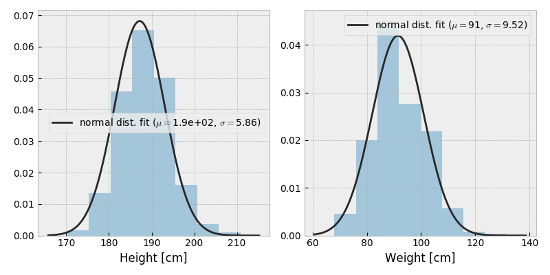 本データを使用した平均身長は 190 cm、平均体重は 91 kg.
身長と体重の箱ひげ図を見てみる.
sns.boxplot(np.char.mod('%.1f', X), Y, color="skyblue")
plt.xticks(rotation=45, fontsize=10, ha='right')
plt.xlabel('Height [cm]')
plt.ylabel('Weight [kg]')
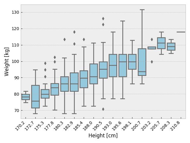 箱の中心線は中央値、箱に含まれる領域にデータの 50% が含まれる. “ひげ”の中には 99.3%のデータが含まれる [Gaussian の場合]. その外側の点は outlier. 分布の非対称性も見て取れる.
次に、散布図の上にプロファイル・プロットを重ね、更にその上に直線フィットの結果を表示する.
plt.scatter(X, Y, alpha=0.2, label='data')

means, means2 = hist.statistic
standard_deviations = numpy.sqrt(means2 - means*means)
bin_edges = hist.bin_edges
bin_centers = (bin_edges[:-1] + bin_edges[1:])/2.
plt.errorbar(x=bin_centers, y=means, yerr=standard_deviations, color='red', linestyle='none',
             marker='o', markersize=8, linewidth=1, capsize=3, alpha=0.5, label='$\mu\pm 1\sigma$ spread')

def linear(x, slope, intercept):
  return x*slope + intercept

from scipy.optimize import curve_fit
popt, pcov = curve_fit(linear, X, Y)

y_lo = linear(X, popt[0]-np.sqrt(pcov[0,0]), popt[1]-np.sqrt(pcov[1,1]))
y_ce = linear(X, popt[0], popt[1])
y_hi = linear(X, popt[0]+np.sqrt(pcov[0,0]), popt[1]+np.sqrt(pcov[1,1]))

plt.plot(X, y_ce, color='red', linewidth=1, alpha=0.5, label='best fit')
plt.plot(X, y_lo, color='red', alpha=0.2, label='$\pm 1\sigma$ band')
plt.plot(X, y_hi, color='red', alpha=0.2)
plt.xlabel('Height [cm]')
plt.ylabel('Weight [kg]')
plt.title('Major League Baseball Players')
plt.legend()
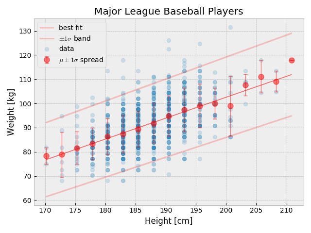 各身長毎の体重の平均値を結ぶ線とフィットの結果は大体一致している. Outliers への対処は行っていないが、損失関数を Huber Loss にしたり、fit の結果を用いて、$\chi^2$ への貢献が大きな点を除いていく等の対処が可能. 本稿では、Bayesian に基づいた outlier の取り扱いを見てみる.
Bayesian approach to outliers
Signal と background を仮定したモデルで、データをフィットする.
\[p(x_i, y_i, e_i | \theta, g_i, \sigma, \sigma_b) = \frac{1 - g_i}{\sqrt{2\pi e_i^2}}\exp\frac{-(y(x_i|\theta)-y_i)^2}{2 e_i^2} + \frac{g_i}{\sqrt{2\pi (e_i^2 + \sigma_b^2)}}\exp\frac{-(\mathcal{N}-y_i)^2}{2 (e_i^2 + \sigma_b^2)}\]\(g_i\) は [0,1] の値を取る nuisance parameter で、0 は signal、1 は background. このモデルを pymc3 で実装し、Markov Chain Monte Carlo (MCMC) を実行する. 体重の誤差は適当に 5 kg としている.
import pymc3 as pm
import theano

S = np.ones(len(X))*5

with pm.Model() as model:
  intercept = pm.Normal('intercept', mu=popt[1], sd=np.sqrt(pcov[1,1]), testval=pm.floatX(0.1))
  slope = pm.Normal('slope', mu=popt[0], sd=np.sqrt(pcov[0,0]), testval=pm.floatX(1.))

  y_s = intercept + slope * X

  y_b = pm.Normal('y_bkgd', mu=0, sd=10, testval=pm.floatX(1.))
  s_b = pm.HalfNormal('s_bkgd', sd=10, testval=pm.floatX(1.))

  frac_noise = pm.Uniform('frac_noise', lower=0.0, upper=.5)
  is_noise = pm.Bernoulli('is_noise', p=frac_noise, shape=len(X),
                           testval=np.random.rand(len(X)) < 0.2)

  yobs = theano.shared(np.asarray(Y, dtype=theano.config.floatX))
  sobs = np.asarray(S, dtype=theano.config.floatX)

  signal = pm.Normal.dist(mu=y_s, sd=sobs).logp(yobs)
  noise = pm.Normal.dist(mu=y_b, sd=sobs + s_b).logp(yobs)
  pm.Potential('obs', ((1 - is_noise) * signal).sum() + (is_noise * noise).sum())

with model:
  traces_signoise = pm.sample(tune=50000)
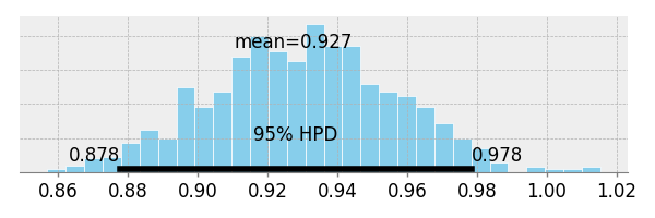
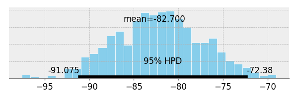
slope と intercept の posterior 分布.
pm.plots.plot_posterior(trace=traces_signoise["slope"])
pm.plots.plot_posterior(trace=traces_signoise["intercept"])
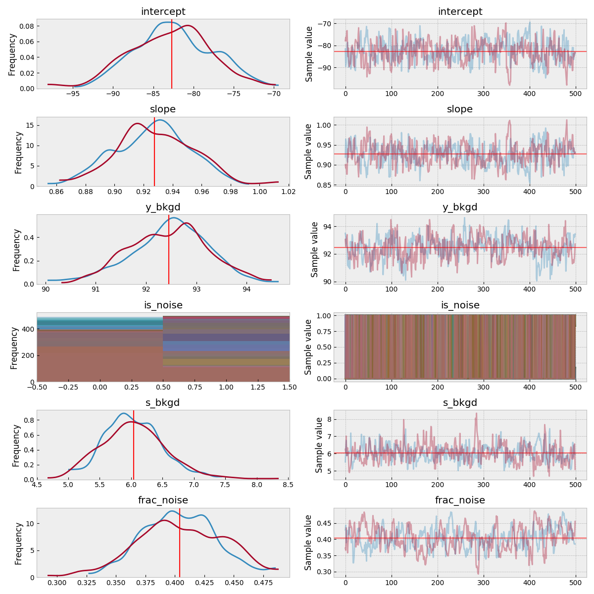
 MCMC の traceplot
pm.traceplot(traces_signoise, figsize=(12, len(traces_signoise.varnames)*1.5),
            lines={k: v['mean'] for k, v in pm.summary(traces_signoise).iterrows()})
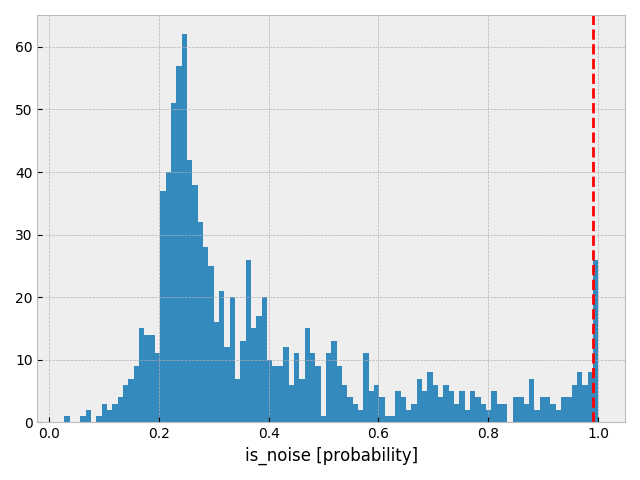
 noise である確率の分布を作成. 確率が 0.99 の場所に赤線を引く.
plt.hist(traces_signoise['is_noise'].sum(axis=0)/1000., bins=100)
plt.axvline(x=0.99, color='r', linestyle='--')
plt.xlabel('is_noise [probability]')
先ほどの linear fit の結果に、Bayesian の結果を重ねる. また、noise である確率が 0.99 以上の点に印を付ける.
def func(x, samp):
 rc = x*samp['slope'] + samp['intercept']
 return rc


pm.plot_posterior_predictive_glm(traces_signoise, lm=func,
        eval=np.linspace(67*inch2cm, 83*inch2cm, 17*inch2cm), samples=200, color='skyblue', alpha=0.5,
        label='MCMC')

plt.scatter(X, Y, alpha=0.2, label='data')
plt.errorbar(x=bin_centers, y=means, yerr=standard_deviations, color='red', linestyle='none',
             #marker='o', markersize=8, linewidth=1, capsize=3, ecolor='red', mfc='none', alpha=0.5)
             marker='o', markersize=8, linewidth=1, capsize=3, alpha=0.5, label='$\mu\pm 1\sigma$ spread')
plt.plot(X, y_ce, color='red', linewidth=1, alpha=0.5, label='best fit')
plt.plot(X, y_lo, color='red', alpha=0.2, label='$\pm 1\sigma$ band')
plt.plot(X, y_hi, color='red', alpha=0.2)

mask = traces_signoise['is_noise'].sum(axis=0)/1000.>=0.99
X_n = X[mask]
Y_n = Y[mask]
plt.scatter(X_n, Y_n, s=50, facecolors='none', edgecolors='r', label='outliers')
plt.xlabel('Height [cm]')
plt.ylabel('Weight [kg]')
plt.title('Major League Baseball Players')
l = plt.legend(fancybox=True)
l.get_frame().set_alpha(0.1)
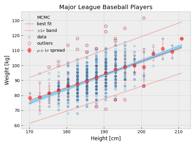
Outlier と判定された点は、linear fit の 1-$\sigma$ band から外れた場所にある. Signal と background をモデル化した Bayesian の fit 結果は単純な linear fit よりも若干傾きが急である. Baysian の方が outlier の取り扱いが elegant な気がするが MCMC は computing intensive で時間が掛かる. 今回の MCMC は、MacBook Air 上で 1時間30分程掛かった.
以上、Bayesian を用いた outliers の取り扱いを見てみた.