Prognostics and health management is an important topic in industry for predicting state of assets to avoid downtime and failures. Public data set for asset degradation modeling from NASA which includes run-to-failure simulated data from turbo fan jet engines is used for prediction of remaining useful life (RUL) of the engines.

Data Set

• A. Saxena and K. Goebel (2008). “Turbofan Engine Degradation Simulation Data Set”, NASA Ames Prognostics Data Repository, NASA Ames Research Center, Moffett Field, CA
• Engine degradation simulation was carried out using C-MAPSS (Commercial Modular Aero-Propulsion System Simulation). Four different sets were simulated under different combinations of operational conditions and fault modes. Records several sensor channels to characterize fault evolution. The data set was provided by the Prognostics CoE at NASA Ames.

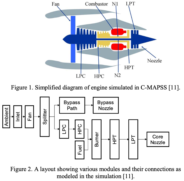
• Engine’s five rotating components: Fan, LPC, HPC (High-Pressure Compressor), HPT (High-Pressure Turbine), LPT
• Gas path: HPC, HPT, LPT
• Operational settings: altitude, throttle resolver angle (TRA), Mach number
• The time series (cycles) of sensed measurements typically available from aircraft gas turbine engines.

Symbol	Description	Units
T2	Total temperature at fan inlet	oR
T24	Total temperature at LPC outlet	oR
T30	Total temperature at HPC outlet	oR
T50	Total temperature at LPT outlet	oR
P2	Pressure at fan inlet	psia
P15	Total pressure in bypass-duct	psia
P30	Total pressure at HPC outlet	psia
Nf	Physical fan speed	rpm
Nc	Physical core speed	rpm
epr	Engine pressure ratio (P50/P2)	–
Ps30	Static pressure at HPC outlet	psia
phi	Ratio of fuel flow to Ps30	pps/psi
NRf	Corrected fan speed	rpm
NRc	Corrected core speed	rpm
BPR	Bypass Ratio	–
farB	Burner fuel-air ratio	–
htBleed	Bleed Enthalpy	–
Nf_dmd	Demanded fan speed	rpm
PCNfR_dmd	Demanded corrected fan speed	rpm
W31	HPT coolant bleed	lbm/s
W32	LPT coolant bleed	lbm/s

a) check input variables

---

def read_data(path):
  df = pd.read_csv(path, delimiter=' ', header=None)
  # check null ratios of each columns
  rc = df.isnull().sum(axis=0)/len(df)
  print(rc[rc!=0.])
  return df

names = ['unit', 'time',
         'altitude', 'mach', 'TRA',
         'T2', 'T24', 'T30', 'T50', 'P2', 'P15', 'P30', 'Nf', 'Nc', 'epr',
         'Ps30', 'phi', 'NRf', 'NRc', 'BPR', 'farB', 'htBleed', 'Nf_dmd', 'PCNfR_dmd', 'W31', 'W32']

df_train = read_data('CMAPSSData/train_FD001.txt')
# remove full of null columns
df_train.drop([26, 27], axis=1, inplace=True)
df_train.columns = names


def inspect_variables(df, unit=None, pdf=None):
  names = df.columns

  nrow = 5
  ncol = 5
  idx = 0
  fig, axes = plt.subplots(nrow, ncol, constrained_layout=True)
  for ii in range(nrow):
    for jj in range(ncol):
      idx = ii*nrow+jj+5
      axes[ii,jj].plot(df[names[idx]][df.unit==unit], marker='o', markersize=1, linewidth=0)
      axes[ii,jj].set_xlabel('{}'.format(names[idx]), fontsize=8)
      if idx==25: break
  fig.suptitle('unit = {}: sensor readings as time series'.format(unit))
  pdf.savefig()
  plt.close()

  fig, axes = plt.subplots(nrow, ncol, constrained_layout=True)
  for ii in range(nrow):
    for jj in range(ncol):
      idx = ii*nrow+jj+5
      axes[ii,jj].hist(df[names[idx]][df.unit==unit], bins=20)
      axes[ii,jj].set_xlabel('{}'.format(names[idx]), fontsize=8)
      if idx==25: break
  fig.suptitle('unit = {}: sensor readings as histogram'.format(unit))
  pdf.savefig()
  plt.close()

  nrow = 2
  ncol = 3
  fig, axes = plt.subplots(nrow, ncol, constrained_layout=True)
  for ii in range(ncol):
    name = names[ii+nrow]
    axes[0,ii].plot(df[name][df.unit==unit], marker='o', markersize=1, linewidth=0)
    axes[0,ii].set_xlabel('time vs {}'.format(name), fontsize=8)
    axes[1,ii].hist(df[name][df.unit==unit], bins=20)
    axes[1,ii].set_xlabel('{} (histogram)'.format(name), fontsize=8)
  fig.suptitle('unit = {}: operational settings'.format(unit))
  pdf.savefig()
  plt.close()


from matplotlib.backends.backend_pdf import PdfPages
with PdfPages('input.pdf') as pdf:
  inspect_variables(df_train, unit=1, pdf=pdf)