c) Feature engineering

Let’s see if linear model can be improved by adding engineered features. Usually we pay more attention to deviations from stable operating conditions. Compute $\phi’$(t) = $\phi$(t) - $\mu(\phi[t_0,t_{19}])$, where $\phi’$ at time step t is derived by subtracting average value of $\phi$ in the first 20 time steps from $\phi$ at time step t. Use both raw and engineered variables for training of linear model. 


---

def feature_engineering(frame):
  window = 20

  df = frame[frame.unit==1].copy()
  stable = df[:window].rolling(window).mean()[-1:]
  features = df - stable.to_numpy()

  for unit in np.arange(2,101):
    df = frame[frame.unit==unit].copy()
    stable = df[:window].rolling(window).mean()[-1:]
    df = df - stable.to_numpy()
    features = pd.concat([features, df])
  diffs = ['unit', 'time', 'altitude', 'mach', 'TRA', 'T2_diff', 'T24_diff', 'T30_diff', 'T50_diff', 'P2_diff',
           'P15_diff', 'P30_diff', 'Nf_diff', 'Nc_diff', 'epr_diff', 'Ps30_diff', 'phi_diff', 'NRf_diff', 'NRc_diff', 'BPR_diff',
           'farB_diff', 'htBleed_diff', 'Nf_dmd_diff', 'PCNfR_dmd_diff', 'W31_diff', 'W32_diff', 'rul']
  features.columns = diffs

  restore = ['unit', 'time', 'rul', 'altitude', 'mach', 'TRA']
  features[restore] = frame[restore]
  return features

features = feature_engineering(train)
df_train = pd.merge(train, features, on=['unit', 'time', 'rul', 'altitude', 'mach', 'TRA'])
x_train, x_val, y_train, y_val = get_train_val(df_train)

reg_lin = LinearRegression()
reg_lin.fit(x_train, y_train)
predictions = reg_lin.predict(x_val)
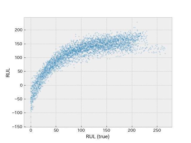
plt.figure()
plt.scatter(y_val, predictions, s=5, alpha=0.2)
plt.xlabel('RUL (true)')
plt.ylabel('RUL')

predictions[predictions < 1] = 1
print('MSE', mean_squared_error(y_val, predictions))
print('R2', r2_score(y_val, predictions))
print('score', custom_loss(y_val, predictions))

Two band structure is not apparent now thanks to feature engineering.

      raw     feature engineered
================================
MSE   1581.6    1190.8
R2    0.57987   0.68369
score inf       inf

Improvements can also be seen in evaluation metrics. RUL prediction has been performed with the simple linear model. Let’s see how more complex models perform with the same data set.